
In the rapidly evolving landscape of data-driven marketing decisions, we’re unveiling the transformative potential of Marketing Mix Modelling (MMM). Whether you’re a seasoned marketer or just starting out, this article serves as your compass to navigate the intricate world of MMM, utilizing the familiar territory of Google Sheets.
Within this article, we walk you through the journey of building a Marketing Mix Model in Google Sheets. From understanding methodology to interpreting statistical results, we’ve got you covered. While the realm of MMM can be intricate, our aim is to simplify the process, ensuring you’re equipped to make informed decisions.
But first things first: To follow along with our article, you can request a link to our template below:
What is Marketing Mix Modelling used for?
Marketing Mix Modelling (MMM), is a tool that helps organizations understand how their marketing efforts influence customer behavior, and how changes to the marketing mix impact business performance.
More concretely, MMM can be used to:
- Optimize marketing mix: Determine the optimal allocation of marketing spend across different marketing channels, products, and regions.
- Evaluate the impact of past marketing initiatives: Assess the effectiveness of past marketing efforts and how they influenced sales or market share.
- Forecast future performance: Predict how changes in the marketing mix will impact sales, market share, and other key performance indicators.
- Allocate budget: Determine the optimal budget allocation for marketing initiatives, taking into account the expected return on investment.
Why Marketing Mix Modelling (MMM)?
As digital advertising and advanced technologies, such as micro-targeting and cookies, grew in popularity, methods like MMM appeared outdated compared to directly tracking individual users to purchase. Nevertheless, with an increase in the use of ad blockers, the implementation of consumer privacy laws like GDPR in Europe or CCPA in California, as well as restrictions on third-party cookies or unique identifiers, there is a shift towards more privacy-sensitive marketing attribution methods. This is why MMM has started to regain its popularity.
What causes fluctuations in our sales?
Although we cannot draw a solid conclusion from our imaginary graph below, we can see fluctuations in sales over time, such as between week 11 and 14.
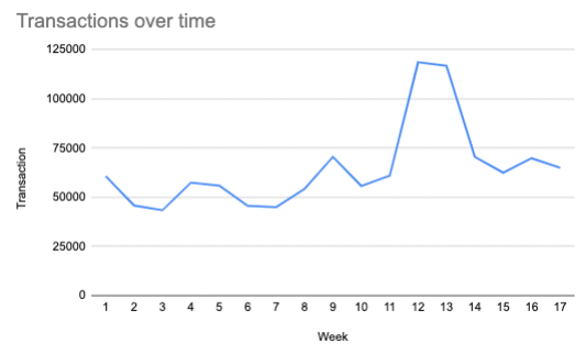
It is in our interest to understand what caused these spikes. Is it external factors? Is it the new awareness campaign that we launched on YT? By better understanding the relation of different variables to sales, we can better evaluate the different channels we are using and allocate our resources accordingly.
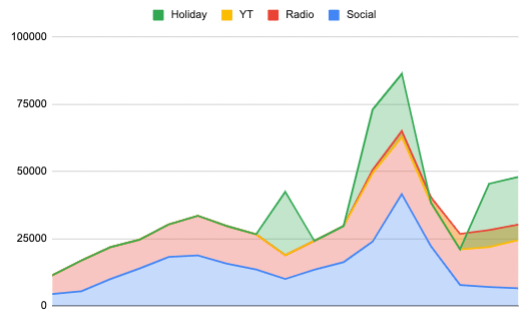
If we use the simple decomposition graph below, we can already see that our first spike in Week 9 was caused by Holidays, whereas the second one was a combination of holidays, radio and social ads.
Methodology
A little forenote, please bear in mind that this is a simplified approach to the infinitely more complicated process of building a solid MMM model. With that said, do not be discouraged and follow along. This will give you the very basics to understand how it works so that when your colleagues start talking about MMM, and trust me they will, you will not be completely clueless on the subject. To read about limitations please visit the ‘limitations’ section.
What we are going to be using to build our model in Google Sheet is the Ordinary Least Squares (OLS), the most popular method for building a linear regression model. It in effect draws a line of best fit between the points of data you have, minimizing the difference between where the line runs and the point on the chart.The ordinary least-squares method is a popular approach for predicting simple linear regression models. It is a simple place to begin with Marketing Mix Modeling, as it can be easily done in a spreadsheet, making it more accessible than more advanced machine learning or Bayesian models.
The purpose of the model is to make the most precise prediction of the dependent variable (such as revenue or conversions) based on the available data of the independent variables, such as advertising spend by channel and organic factors like seasonality or national holidays. Once the model is developed and validated, it can be utilized to calculate the impact of each media channel (how many sales would not have happened without advertising?), as well as to predict future advertising budget allocation (what will happen if you double your advertising budget?).
A simple linear regression formula for a model with just one media channel and one organic variable appears as follows:
Y = B2X2 + B1X1 + B0
Where:
- Y represents the revenue from sales or number of conversions.
- B2 represents the coefficient for advertising, meaning how many sales are generated per dollar spent.
- X2 represents the amount of money spent on advertising.
- B1 represents the coefficient for an organic variable, such as Google search trends in the industry.
- X1 represents the value of an organic variable, like an index of Google search trends ranging from 0 to 100.
- B0 represents the intercept, or the number of sales that would occur if no money was spent on advertising and there was no contribution from organic variables.
As previously stated, this is a simplified version of more complex models. If you are interested in building a more accurate and complex model, you can use open-source libraries like Robyn by Meta, or LightweightMMM by Google, but you’ll likely need a Data Scientist. In case you need help with building and interpreting your MMM model, you can refer to our sister company LYKTA.
How can we do Media Mix Modelling in Google Sheets?
1) Get your data
Below you will find a simplified version of the data that you will need:
- Column 1: Time variable (Days or weeks)
- Column 2: Variable that you are trying to predict (generally revenue or sales)
Following columns, the variables that might have had an impact on your business e.g. Media Spending, Holidays, Price, Promotions.
Nevertheless, obtaining reliable data, particularly media spending, is not always a straightforward process.
As a media company, we can attest that obtaining net media spending is not as simple as it may seem. There are various factors to consider, such as how to deal with sponsoring costs or packages, such as Auvio or RTL Play. These costs can be challenging to isolate from the overall media spend and can skew the results of the modeling if not accounted for accurately.
Furthermore, traditional media channels such as print and Out of Home (OOH) advertising can be tricky to split per day. This poses a challenge for businesses that want to understand the effect of their advertising spend on sales on a daily basis.
Despite these challenges, obtaining accurate data is critical to the success of MMM. Without reliable data, the modeling results may be misleading and result in ineffective marketing strategies.
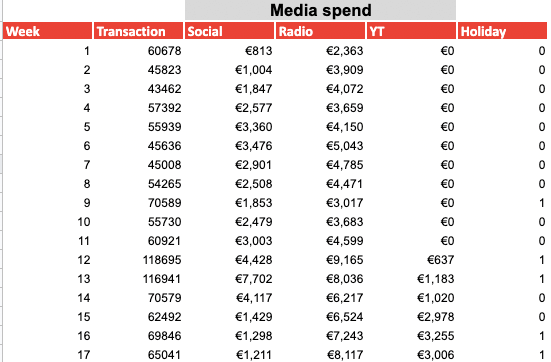
Not all variables need to be your regular channels as your sales may be related to external factors. This is why we have added a column called Holidays. Ideally, this would help us build a better model if it did impact on business.
2) Check your data
The second step of the process involves data checking, which includes identifying missing values and managing them appropriately. It is crucial to note that a value of zero does not necessarily mean that the data is unavailable. Thus, it is essential to differentiate between zero values and missing data.
Moreover, to ensure accurate results, it is essential to check for correlations between the variables. If two variables are highly correlated, it can lead to misleading results, as the effect of one variable cannot be isolated from the other. For example, if a business invests in Facebook and TV advertising simultaneously, it becomes challenging to separate their effects on the outcome.
Furthermore, businesses can derive additional data by incorporating seasonality data into the analysis. This helps account for any seasonal changes that may affect the outcome.
In conclusion, the second step of the market mix modelling process involves thorough data checking, including managing missing values, checking for correlations between variables, and incorporating seasonality data. By ensuring the quality of the data, businesses can achieve accurate results that inform their marketing strategies effectively.
3) Multi-Linear regression
The correlation coefficient and R^2 (coefficient of determination) are important measures in linear regression analysis, as they help to evaluate the strength and direction of the linear relationship between the independent and dependent variables (More info in the ‘Statistical Verification’ section).
The correlation coefficient (r) indicates the strength and direction of the linear relationship between two variables, and it ranges from -1 to 1. A value of -1 indicates a perfect negative linear relationship, a value of 0 indicates no linear relationship, and a value of 1 indicates a perfect positive linear relationship. The correlation coefficient can help identify whether the relationship between the variables is strong or weak and whether it is a positive or negative relationship.
The coefficient of determination (R^2) is a measure of how well the regression line (or model) fits the data. It represents the proportion of the variation in the dependent variable that is explained by the independent variable. It ranges from 0 to 1, with a value of 1 indicating that the model explains all the variation in the dependent variable. R^2 can help evaluate how well the linear regression model fits the data and how much of the variation in the dependent variable is accounted for by the independent variable.
In order to establish our statistical metrics such as correlation coefficient or R^2, we will use the following function:
=LINEST(Know_data_y, Known_data_x, , [calculate_b], [verbose])
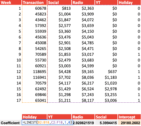
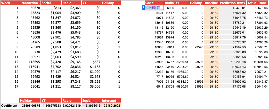
By inputting 0 as verbose, we only obtain the correlation coefficient of the different variables as well as the intercept, which we will then use to build our model. Be aware that the coefficient comes out in order, so our last variable Holiday is now the first variable.
Now that we have the correlation coefficient, as per formula Y = B2X2 + B1X1 + B0, we need to:
- Multiply each variable by its coefficient
- Sum them together
- Add the intercept
4) Checking the verbose output of our statistics
As you see below, if we input 1 as a verbose output, Google Sheets provides us with several statistical metrics that we can then use to test the validity of our model (more details in the ‘Statistical Verification’ section).
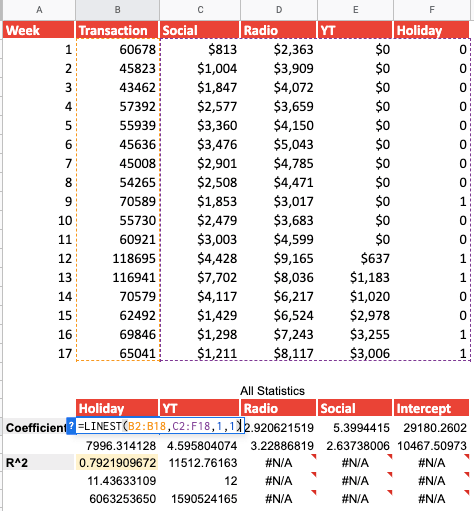
What we are interested in for now, beside the coefficient that we already have, is the R^2. This number demonstrates to what extent our model explains the variance that we see in sales, which in this case is 0.79 (Please refer to the ‘Statistical Verification’ section to find out how to interpret statistical metrics). If you are wondering why we have N/A, it is inevitable as there is no data to be shown for those cells.
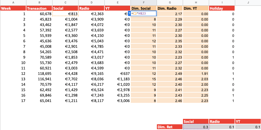
5) Calculating Adstock
Adstock is a term used in advertising to quantify the residual impact of previous advertising efforts. For instance, if a company launches an advertising campaign in week 1, there will be a portion of that level that remains in week 2. In week 3, there will be a portion of the level from week 2. Essentially, Adstock represents the gradual decrease in the impact of advertising over time, expressed as a percentage.
The formula is:
At = Xt + Adstock rate * At-1
Where:
- At-1 = the previously calculated Adstock
- Xt = Advertising spent
- Adstock rate = Percentage of residual impact of previous Adstock
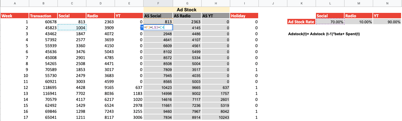
Using this formula, we are now able to calculate the individual channels’ Adstock. Using the LINEST function we can then calculate the coefficient between our new variables, i.e. AS Social, AS Radio, AS YT, and the transactions, to create new predictions. If we look at our new R^2 we see that this has increased from 79.12% to 80.07%. Depending on the model and the variable you use, Adstock can have a different impact, or no impact at all.
6) Calculating the ideal Adstock rate
If you are wondering how to calculate the optimal Adstock rate which maximizes your R^2, you can either play around with it to see how it impacts your R2 or simply use Excel. Unfortunately this function does not exist in GSheet that I know of – if you do please feel free to leave it in the comment below.
Let’s see how this can be done in excel. Firstly, download the file and open it in excel. Navigate to Data → Solver.

A pop up window will open where you can set the parameters to maximize your R^2.
- As an objective, select the cell where your R^2 is.
- Click on “Max” as this is the metric you want to maximize.
- By Changing Variable Cells: Select the cell where your Adstock rate is (multiple cells if you have multiple Adstock rates).
- Subject to constraints → Add → Select your cells with your Adstock rate and select lower than 1 and higher than 0.
- Click on Solve.
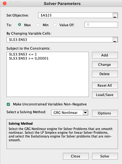
Excel will change the Adstock rate until it has found the one that optimizes your R^2 and therefore your model accuracy. When using more advanced machine learning tools like we do at LYKTA, the rate is automatically calculated for you.
7) Calculating Diminishing Returns & Saturation
Diminishing Returns refers to the idea that the marginal benefit of advertising decreases as more is spent. In other words, doubling the amount spent on advertising does not necessarily double the sales. This is because there is a point of saturation, where additional advertising has little to no impact on sales. For this we use the power function formula:
y = α⋅x^B ; 0 < B ≤ 1
Where:
- Y represents the revenue from sales or number of conversions.
- α represents the correlation coefficient.
- X represents your spend.
- B represents your “Saturation rate”.
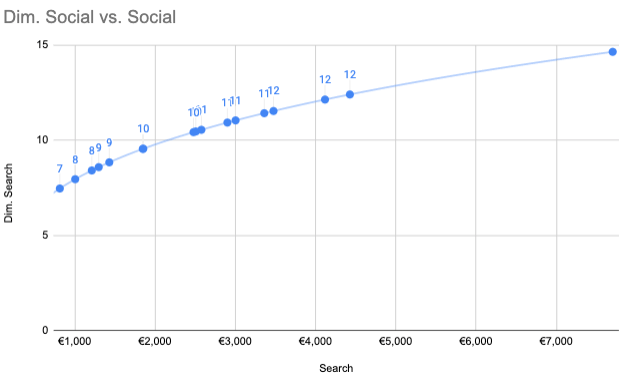
Using this formula, we can now calculate the individual channels’ saturation. Using the LINEST function we can then calculate the coefficient between our new variables and the transactions to create new predictions.
The image below graphically shows the concept of Diminishing Returns. With the first 2K spent we generated 10 conversions, whereas to generate just 1 incremental conversion we had to spend 1K extra.
8) Transformed Linear Regression
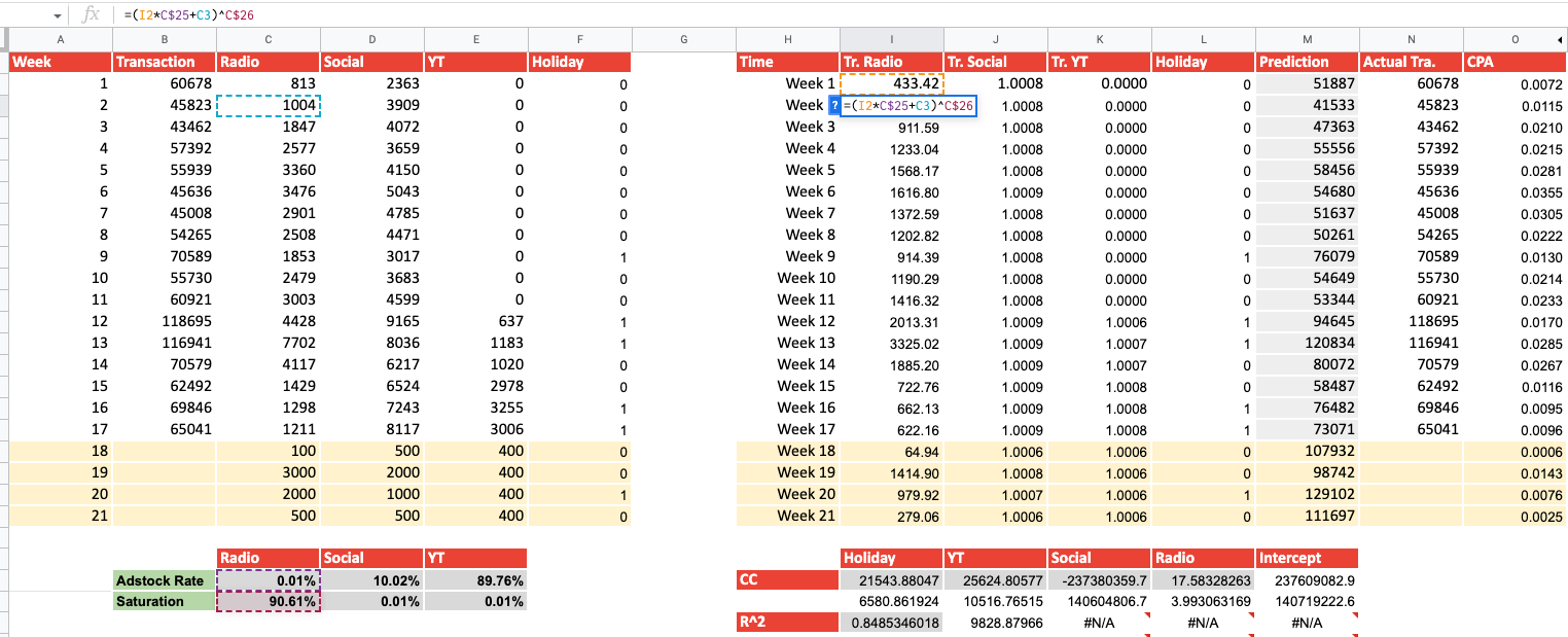
Using Diminishing Return and Adstock combined we can try to build a more accurate model. We can use the formula
Y= (Xt + Adstock rate * At-1)^β ; 0 < β ≤ 1.
![]()
Always remember to evaluate or model for accuracy and statistical significance. (Visit the ‘Statistical Verification’ section for more info)
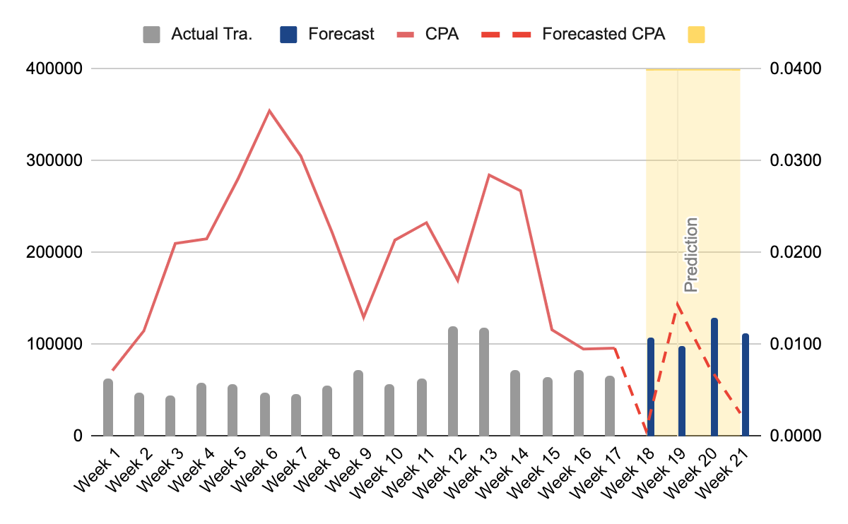
9) Prediction and Budget Allocation
If you are satisfied with your model’s accuracy and your variables are statistically significant, you can now make predictions and see how your budget allocation influences your transactions and CPA. Using the previously mentioned formula, assign different budget to the channels and see the effects for yourself:
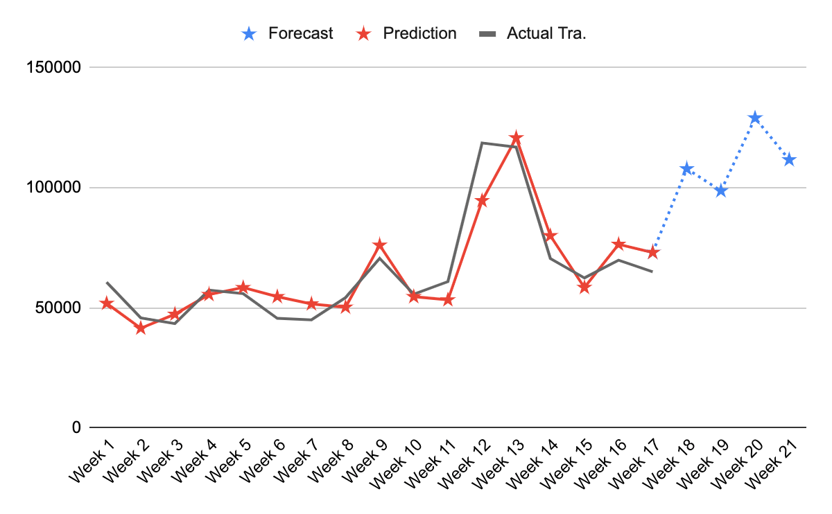
If you are presenting this to someone, remember that a graph can go a long way:
10) Statistical Verification
The following can be used to verify the statistical validity and accuracy of your model:
- The LINEST function.
- The difference between your actual sales (or conversions).
- Your prediction.
According to the outcome of your statistical verification you can then modify the model accordingly by excluding the variables that are not significant or adding new variables.
By using the LINEST function, you will be able to calculate your P-value and establish the statistical validity of your variables.The difference between predictions and actual sales, called error, will allow you to calculate important metrics such as MAPE and NRMSE. Please check out the template to see the formulas in detail.
Bear in mind that to keep things simple we only have one with data in our template, however if the goal is to predict future sales accurately, it is crucial to split the data into three categories: train data, validation, and test. If you are interested in finding out more about how to build a model I suggest having a look at How to Build your MMM at Vexpower.com.
The train data is used to build the model, while the validation data is used to fine-tune the model and make any necessary adjustments. The test data is then used to evaluate the accuracy of the model.
Splitting the data into these categories is a best practice for MMM as it helps avoid overfitting, which occurs when the model is too closely tailored to the training data and does not generalize well to new data. Overfitting can lead to misleading results and ineffective marketing strategies.
By evaluating the model’s accuracy on the test set, businesses can ensure that the model is not just effective for the analyzed period but can also generalize well to future periods.
Another important statistical measurement is the RSSD, used to calculate the “plausibility” of your model. To keep things simple, we did not cover this in the model.
Interpreting your statistical results
R^2
- R^2 < 0.8 = Not good
- 0.8 < R^2 < 0.9 = Acceptable
- R^2> 0.9 = Great
NRMSE – Normalized Root Mean Square Error
- RMSE > 0.1 = Not good
- 0.1 < RMSE< 0.05 = Acceptable
- RMSE<0.05 = Great
MAPE – Mean Absolute Error
- MAPE > 10% = Not good
- 10%< MAPE< 5% = Acceptable
- MAPE <5% = Great
In hypothesis testing, the p-value is used to assess the evidence against the null hypothesis (H0). If the p-value is less than a predetermined level of significance (often represented by alpha, denoted as α), it is considered statistically significant and suggests that the null hypothesis should be rejected. In this case, you would accept the alternative hypothesis (H1).
In other words, if the p-value is less than alpha (p < α), it means that the results are unlikely to have occurred by chance and provide evidence against the null hypothesis. This means that you can conclude that the alternative hypothesis is supported by the data and is likely to be true.
For example, if alpha is set at 0.05, and the p-value is 0.03, it suggests that there is less than a 5% chance that the observed results could have happened by chance if the null hypothesis were true. In this case, you would reject the null hypothesis and accept the alternative hypothesis.
To sum it up:
For α=0.05
- P-Value> 0.05 = Not significant
- P-Value<0.05 = Significant at 95%
11) Limitations
Simple linear regression makes the assumption that the effectiveness of marketing efforts does not change over time, which can lead to inaccurate results such as attributing negative sales to certain channels. In these cases, it is recommended to use more advanced techniques.
It is possible that you may not have access to all the necessary data to create a precise and reliable model. This is a common issue, especially if you haven’t spent enough time collecting data, which can take several weeks or even months depending on the size and complexity of your business, or if some of the variables that affect your marketing performance are difficult to measure.
It’s essential to be careful when building a model, as the wrong model can lead to costly decisions. It’s always a good idea to consult with a statistician or business analyst who has econometrics and data science expertise, or to learn more about MMM before making any important and irreversible decisions using this method.As a final note, I want to give credit to Michael Taylor as this model was developed thanks to his course on MMM model building on Vexpower.
If you are interested in a more elaborate MMM model in GSheet, you can check this out.
If you are interested in having your model built by a professional do not hesitate to get in contact with LYKTA.
Recevez notre newsletter &
nos insights
Nous approfondissons les sujets brûlants du marketing numérique et aimons partager.